install.packages("ecoengine", dependencies = TRUE)
# Requires R version 3.0.1 or higher
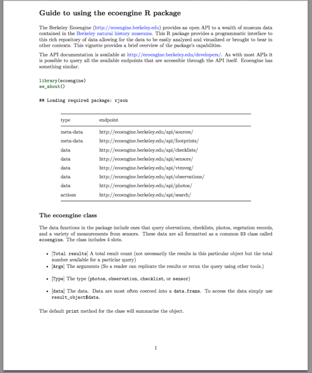
library(ecoengine)
ee_about()
##        type                                        endpoint
## 1 meta-data      http://ecoengine.berkeley.edu/api/sources/
## 2 meta-data   http://ecoengine.berkeley.edu/api/footprints/
## 3      data   http://ecoengine.berkeley.edu/api/checklists/
## 4      data      http://ecoengine.berkeley.edu/api/sensors/
## 5      data       http://ecoengine.berkeley.edu/api/vtmveg/
## 6      data http://ecoengine.berkeley.edu/api/observations/
## 7      data       http://ecoengine.berkeley.edu/api/photos/
## 8   actions       http://ecoengine.berkeley.edu/api/search/
source_list <- ee_sources()
unique(source_list$name)
##  [1] "LACM Vertebrate Collection"
##  [2] "MVZ Birds"
##  [3] "MVZ Herp Collection"
##  [4] "MVZ Mammals"
##  [5] "Wieslander Vegetation Map"
##  [6] "CAS Herpetology"
##  [7] "Consortium of California Herbaria"
##  [8] "UCMP Vertebrate Collection"
##  [9] "Sensor Data Qualifiers"
## [10] "Essig Museum of Entymology"
results <- ee_observations(genus = "Lynx", progress = FALSE)
results
## [Total results]: 795
## [Args]:
## country = United States
## genus = Lynx
## georeferenced = FALSE
## page_size = 25
## page = 1
## [Type]: observations
## [Number of results]: 25
results <- ee_observations(genus = "Lynx", page = 1:2, progress = FALSE)
results
## [Total results]: 795
## [Args]:
## country = United States
## genus = Lynx
## georeferenced = FALSE
## page_size = 25
## page = 1 2
## [Type]: observations
## [Number of results]: 50
pinus_observations <- ee_observations(scientific_name = "Pinus", page = 1, quiet = TRUE,
    progress = FALSE)
pinus_observations
## [Total results]: 48333
## [Args]:
## country = United States
## scientific_name = Pinus
## georeferenced = FALSE
## page_size = 25
## page = 1
## [Type]: observations
## [Number of results]: 25
animalia <- ee_observations(kingdom = "Animalia")
Artemisia <- ee_observations(scientific_name = "Artemisia douglasiana")
asteraceae <- ee_observationss(family = "asteraceae")
vulpes <- ee_observations(genus = "vulpes")
Anas <- ee_observations(scientific_name = "Anas cyanoptera", page = "all")
loons <- ee_observations(scientific_name = "Gavia immer", page = "all")
plantae <- ee_observations(kingdom = "plantae")
# grab first 10 pages (250 results)
plantae <- ee_observations(kingdom = "plantae", page = 1:10)
chordata <- ee_observations(phylum = "chordata")
# Class is clss since the former is a reserved keyword in SQL.
aves <- ee_observations(clss = "aves")
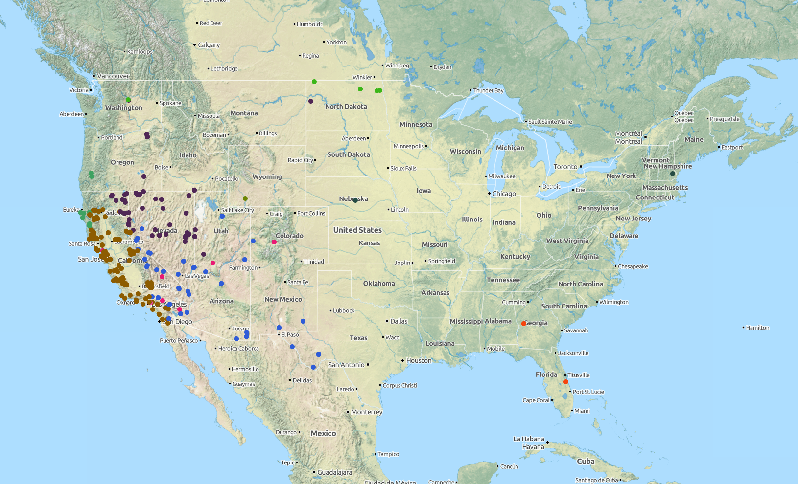
lynx_data <- ee_observations(genus = "Lynx", georeferenced = TRUE, page = "all",
    quiet = TRUE)
ee_map(lynx_data)
head(ee_list_sensors())
##            station_name                       units
## 1          Angelo HQ WS Kilojoules per square meter
## 2      Angelo Meadow WS      Watts per square meter
## 3 Angelo HQ SF Eel Gage                     Percent
## 4          Angelo HQ WS                      Degree
## 5         Cahto Peak WS           Meters per second
## 6      Angelo Meadow WS           Meters per second
##                       variable                       method_name record
## 1 Solar radiation total kj/m^2 Conversion to 30-minute timesteps   1625
## 2  Solar radiation total w/m^2 Conversion to 30-minute timesteps   1632
## 3            Rel humidity perc Conversion to 30-minute timesteps   1641
## 4       Wind direction degrees Conversion to 30-minute timesteps   1644
## 5            Wind speed avg ms Conversion to 30-minute timesteps   1651
## 6            Wind speed max ms Conversion to 30-minute timesteps   1654
# First we can grab the list of sensor ids
sensor_ids <- ee_list_sensors()$record
# In this case we just need data for sensor with id 1625
angelo_hq <- sensor_ids[1]
results <- ee_sensor_data(angelo_hq, page = 2, progress = FALSE)
results
## [Total results]: 56779
## [Args]:
## page_size = 25
## page = 2
## [Type]: sensor
## [Number of results]: 25
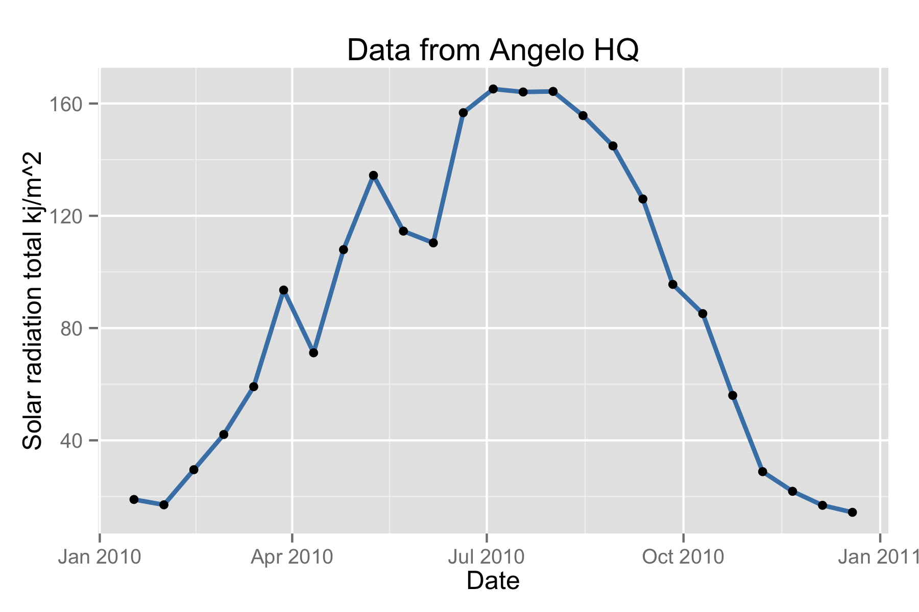
stations <- ee_list_sensors()
sensor_df <- ee_sensor_agg(sensor_id = stations[1, c("record")], weeks = 2,
    progress = FALSE)
head(sensor_df$data)
##    begin_date  mean min   max   sum count
## 2  2010-01-17 18.94   0 150.8  7613   402
## 26 2010-01-31 17.03   0 237.7 11444   672
## 3  2010-02-14 29.54   0 336.3 19852   672
## 4  2010-02-28 42.08   0 402.5 28276   672
## 5  2010-03-14 59.12   0 466.6 39730   672
## 6  2010-03-28 93.55   0 490.6 62678   670
rodent_pages <- ee_pages(ee_observations(order = "Rodentia", progress = FALSE,
    quiet = TRUE))
page_breaks <- split(1:rodent_pages, ceiling(seq_along(1:rodent_pages)/1000))
rodent_data <- list()
# This step will take a while, as it downloads ~50 mb of data with pauses to
# avoid hammering API
for (i in 1:length(rodent_data)) {
    rodent_data <- ee_observations(order = "Rodentia", page = page_breaks[[1]])
    write.csv(rodent_data$data, file = paste0("rodent_data", i, ".csv"))
}
library(plyr)
rodent_pages <- ee_pages(ee_observations(order = "Rodentia", progress = FALSE,
    quiet = TRUE))
page_breaks <- split(1:rodent_pages, ceiling(seq_along(1:rodent_pages)/1000))
results <- ldply(page_breaks, function(x) {
    results <- ee_pages(ee_observations(order = "Rodentia", page = x, quiet = TRUE))
    results$data
}, .progress = "text")
library(dplyr)
rodents_summary <- rodents %.% filter(!is.na(year)) %.% group_by(state = abbreviation,
    year) %.% summarise(counts = n())
head(rodents_summary)
##   State Year Counts
## 1    CA 1818      9
## 2    OR 1899     16
## 3    CA 1904    178
## 4    OR 1905     32
## 5    CA 1905     18
## 6    CA 1907     32
library(rMaps)
rodents_summary <- dplyr::filter(rodents_summary, Year > 1899)
ichoropleth(Counts ~ State, data = rodents_summary, animate = "Year", pal = "Reds",
    ncuts = 4, play = TRUE)
all_lists <- ee_checklists()
nrow(all_lists)
## [1] 57
unique(all_lists$subject)
##  [1] "Mammals"                  "Mosses"
##  [3] "Beetles"                  "Spiders"
##  [5] "Amphibians"               "Ants"
##  [7] "Fungi"                    "Lichen"
##  [9] "Plants"                   "Reptiles"
## [11] "Algae"                    "Arthropods"
## [13] "Liverworts"               "Birds"
## [15] "Butterflies & Moths"      "Fish"
## [17] "Bees"                     "Archaeognatha"
## [19] "Insects 1937-1955"        "Orthoptera and Cicadidae"
## [21] "Butterflies"              "Aquatic Insects"
## [23] "Stoneflies"               "Caddisflies"
## [25] "whipworms"                "Tardigrades"
## [27] "Small Mammals"            "False Scorpions"
## [29] "Crane-flies"              "Chiggers"
## [31] "Cestodes"                 "Rodents"
## [33] "Lichens"                  "Grasses and Forbes"
## [35] "Macroinvertebrates"       "Amphibians and Reptiles"
spiders <- ee_checklists(subject = "Spiders")
spiders
##                  record
## 4  bigcb:specieslist:15
## 10 bigcb:specieslist:20
##                                                         footprint
## 4  http://ecoengine.berkeley.edu/api/footprints/hastings-reserve/
## 10   http://ecoengine.berkeley.edu/api/footprints/angelo-reserve/
##                                                                       url
## 4  http://ecoengine.berkeley.edu/api/checklists/bigcb%3Aspecieslist%3A15/
## 10 http://ecoengine.berkeley.edu/api/checklists/bigcb%3Aspecieslist%3A20/
##                                           source subject
## 4  http://ecoengine.berkeley.edu/api/sources/18/ Spiders
## 10 http://ecoengine.berkeley.edu/api/sources/18/ Spiders
library(plyr)
spider_details <- ldply(spiders$url, checklist_details)
names(spider_details)
##  [1] "url"                              "observation_type"
##  [3] "scientific_name"                  "collection_code"
##  [5] "institution_code"                 "country"
##  [7] "state_province"                   "county"
##  [9] "locality"                         "coordinate_uncertainty_in_meters"
## [11] "begin_date"                       "end_date"
## [13] "kingdom"                          "phylum"
## [15] "clss"                             "order"
## [17] "family"                           "genus"
## [19] "specific_epithet"                 "infraspecific_epithet"
## [21] "source"                           "remote_resource"
## [23] "earliest_period_or_lowest_system" "latest_period_or_highest_system"
photos <- ee_photos(quiet = TRUE, progress = FALSE)
photos
## [Total results]: 43708
## [Args]:
## page_size = 25
## georeferenced = 0
## page = 1
## [Type]: photos
## [Number of results]: 25
view_photos()
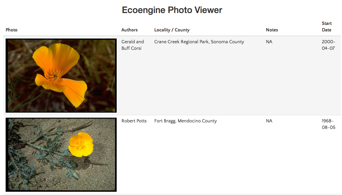
poppys <- ee_photos(scientific_name = "Eschscholzia californica", quiet = TRUE,
    progress = FALSE)
view_photos(poppys)
/
#